Many social media platforms such as Facebook [1], LinkedIn [2], and Twitter [3] have standard guidelines to enforce integrity and make their platforms safe for users. These guidelines prohibit certain user behaviors, activities, and content that are harmful to the community. It is essential to have technologies and resources in place to identify harmful content and bad actors. We can divide the focus of integrity enforcement into two categories:
- Harmful content: Posts that contain violence, nudity, self-harm, hate speech, etc.
- Bad acts/bad actors: Fake accounts, spam, phishing, organized unethical activities, and other unsafe behaviors.
In this chapter, we focus on detecting posts that might contain harmful content. In particular, we design a system that proactively monitors new posts, detects harmful content, and removes or demotes them if the content violates the platform's guidelines. To understand how companies build a harmful content detection system in practice, refer to [4] [5] [6].
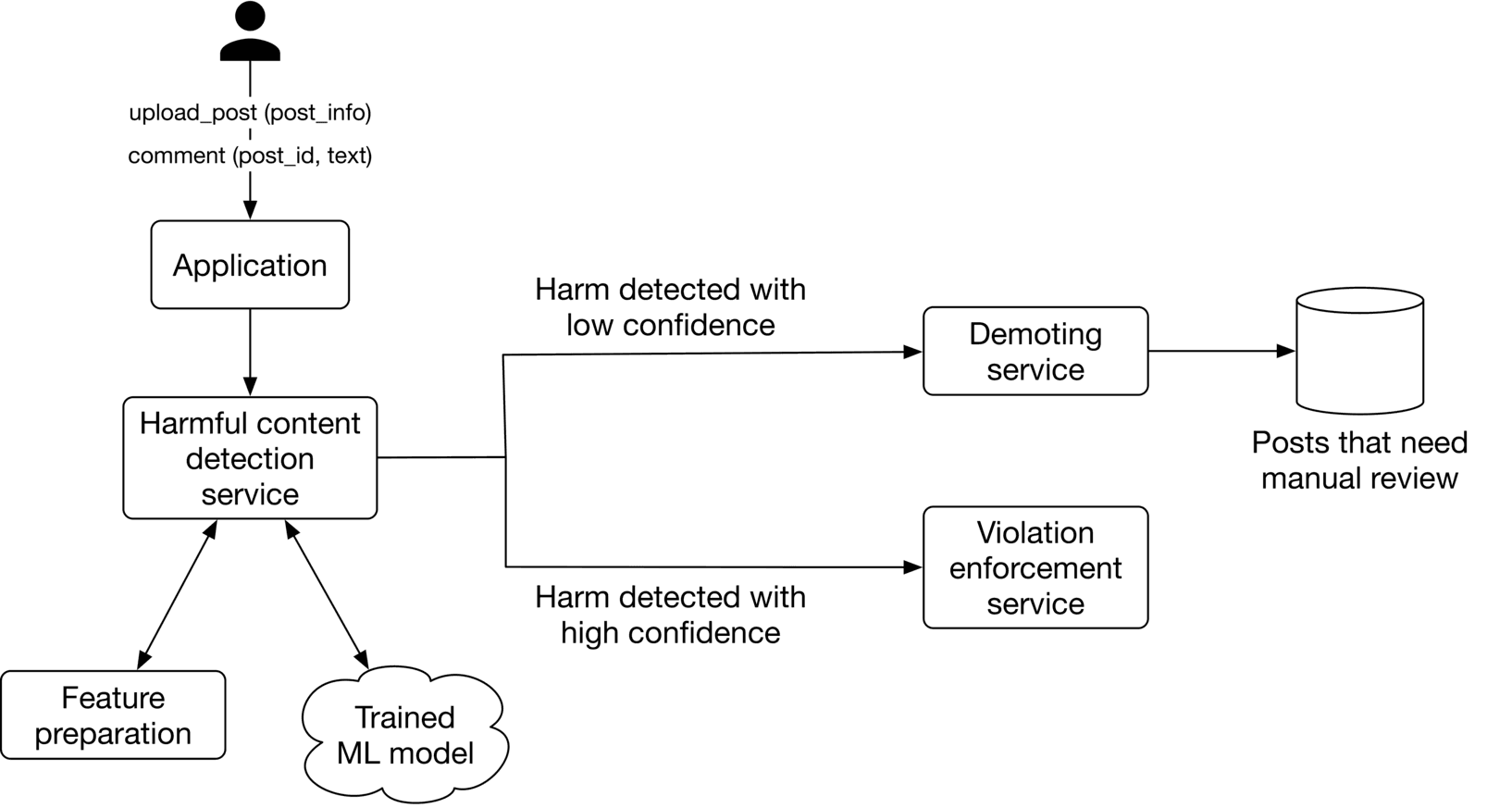 Figure 5.1: Harmful content detection system
Clarifying Requirements
Here is a typical interaction between a candidate and an interviewer.
Candidate: Does the system detect both harmful content and bad actors?
Interviewer: Both are equally important. For simplicity, let's focus on detecting harmful content only.
Candidate: Should a post only contain text, or are images and videos allowed?
Interviewer: The content of a post can be text, image, video, or any combination of these.
Candidate: What languages are supported? Is it English only?
Interviewer: The system should detect harmful content in various languages. For simplicity, assume we can use a pre-trained multilingual model to embed the textual content.
Candidate : Which specific categories of harmful content are we looking to identify? I can think of violence, nudity, hate speech, misinformation, etc. Are there other harmful categories to consider?
Interviewer: Great, you brought up the major ones. Misinformation is more complex and controversial. For simplicity, let's not focus on misinformation.
Candidate : Are there any human annotators available to label posts manually?
Interviewer: The platform receives more than 500 million posts each day. Asking humans to label all of them would be very expensive and time-consuming. However, you can assume human annotation is available to label a limited number of posts, say 10,000 per day.
Candidate: Allowing users to report harmful content is beneficial for understanding where the system is failing. Can I assume the system has that feature?
Interviewer: Good point. Yes, users can report harmful posts.
Candidate: Should we explain why a post is deemed harmful and removed?
Interviewer: Yes. Explaining to users why we remove a post is essential. It helps users to ensure they align their future posts with the guidelines.
Candidate: What is the system's latency requirement? Do we need a real-time prediction, i.e., the system detects harmful content immediately and blocks it, or can we rely on batch prediction, i.e., detecting harmful content offline hourly or daily?
Interviewer: This is a very important question. What are your thoughts?
Candidate: In my opinion, the requirements for different harmful content might vary. For example, violent content may require real-time solutions, while for others, late detection may work.
Interviewer: Those are fair assumptions.
So, let's summarize the problem statement. We will design a harmful content detection system, which identifies harmful posts, then deletes or demotes them and informs the user why the post was identified as harmful. A post's content can be text, image, video, or any combination of these, and the content can be in different languages. Users can report harmful posts.
Frame the Problem as an ML Task
Defining the ML objective
We define our ML objective as accurately predicting harmful posts. The reason is that if we can accurately detect harmful posts, we can remove or demote them, leading to a safer platform.
Specifying the system's input and output
The system receives a post as input, and outputs the probability that the post is harmful.
Figure 5.2: A harmful content detection system’s input-output
Let’s dive deeper into the input post. As shown in Figure 5.3, a post can be heterogeneous and potentially multimodal.
Figure 5.3: Heterogeneous post data
To make accurate predictions, the system should consider all modalities. Let's discuss two commonly used fusing methods to combine heterogeneous data: late fusion and early fusion.
Late fusion
With late fusion, ML models process different modalities independently, then combine their predictions to make a final prediction. The figure below illustrates how late fusion works.
Figure 5.4: Late fusion
The advantage of late fusion is that we can train, evaluate, and improve each model independently.
However, late fusion has two major disadvantages. First, to train these individual models, we need to have separate training data for each modality, which can be time-consuming and expensive.
Second, the combination of the modalities might be harmful, even if each is benign in isolation. This is frequently the case with memes that combine images and text. In these cases, late fusion fails to predict whether the content is harmful. This is because each modality is benign, so the models predict benignity when processing each modality. The fusion layer output is benign because the output of each separate modality is benign. But this is incorrect, as the combination of modalities can be harmful.
Early fusion
With early fusion, the modalities are combined first, and then the model makes a prediction. Figure 5.5 illustrates how early fusion works.
Figure 5.5: Early fusion
Early fusion has two major advantages. First, it is unnecessary to collect training data separately for each modality. Since there is a single model to train, we only need to collect training data for that model. Second, the model considers all the modalities, so if each modality is benign, but their combination is harmful, then the model can potentially capture this in the unified feature vector.
However, learning this task is more difficult for the model due to the complex relationships between modalities. In the absence of sufficient training data, it is challenging for the model to learn complex relationships and make good predictions.
Which fusion method should we use?
The early fusion method is used because it allows us to capture posts that may be harmful overall, even if each modality is benign on its own. Additionally, with around 500 million posts being published every day, the model has enough data to learn the task.
Choosing the right ML category
In this section, we examine the following ML category options:
- Single binary classifier
- One binary classifier per harmful class
- Multi-label classifier
- Multi-task classifier
Single binary classifier
In this option, a model takes the fused features as input and predicts the probability of the post being harmful (Figure 5.6). Since the output is a binary outcome, the model is a binary classifier.
Figure 5.6: A single binary classifier
The shortcoming of this option is that it's difficult to determine which class of harm, such as violence, a post belongs to. This limitation causes two main issues:
- It is not easy to inform users why we take down a post as the system only outputs a binary value indicating whether the post as a whole is harmful or not. We have no clue which particular class of harm the post belongs to.
- It is not easy to identify harmful classes in which the system doesn't perform well, meaning we cannot improve the system for underperforming classes.
Since it is essential to explain why a post is removed, a single binary classifier is not a good option.
One binary classifier per harmful class
In this option, we adopt one binary classifier for each harmful class. As Figure 5.75.75.7 shows, each model determines if a post belongs to a specific harmful class or not. Each model takes fused features as input and predicts the probability of the post being classified as a harmful class.
Figure 5.7: One binary classifier per harmful class
The advantage of this option is that we can explain to users why a post was taken down. In addition, we can monitor different models and improve them independently.
However, this option has one major drawback. Since we have multiple models, they must be trained and maintained separately. Training these models separately is time-consuming and expensive.
A multi-label classifier
In multi-label classification, the data point we want to classify may belong to an arbitrary number of classes. In this option, a single model is used as a multi-label classifier. As Figure 5.85.85.8 shows, the input to the model is the fused features, and the model predicts probabilities for each harmful class.
Figure 5.8: A multi-label classifier
By using a shared model for all harmful classes, training and maintaining the model is less costly. If you would like to learn more about this method, refer to the approach called WPIE [7].
However, predicting the probabilities of each harmful class using a shared model isn’t ideal, as the input features may need to be transformed differently.
Multi-task classifier
Multi-task learning refers to the process in which a model learns multiple tasks simultaneously. This allows the model to learn similarities between tasks. By doing so, we avoid unnecessary computations when a certain input transformation is beneficial for multiple tasks.
In our case, we treat different classes of harm, such as violence and nudity, as different tasks and use a multi-task classification model to learn each task. As Figure 5.9 shows, multi-task classification has two stages: shared layers and task-specific layers.
Figure 5.9: Multi-task classification overview
Shared layers A shared layer, as shown in Figure 5.10, is a set of hidden layers that transform input features into new ones. These newly transformed features are used to make predictions for each of the harmful classes.
Figure 5.10: Shared layers
Task-specific layers Task-specific layers are a set of independent ML layers (also called classification heads). Each classification head transforms features in a way that is optimal for predicting a specific harm probability.
Figure 5.11: Task-specific layers
Multi-task classification has three advantages. First, it is not expensive to train or maintain since we use a single model. Second, the shared layers transform the features in a way that is beneficial for each task. This prevents redundant computations and makes multi-task classification efficient. Lastly, the training data for each task contributes to the learning of other tasks. This is especially helpful when limited data is available for a particular task.
Because of these advantages, we employ a multi-task classification method. Figure 5.125.125.12 shows how we frame the problem.
Figure 5.12: Frame the problem as an ML task
Data Preparation
Data engineering
We have the following data available:
- Users
- Posts
- User-post interactions
Users
A user data schema is shown below.
| ID | Username | Age | Gender | City | Country | |
|---|---|---|---|---|---|---|
| Table 5.1: User data schema |
Posts
Post data contain fields such as author, time of upload, etc. Table 5.25.25.2 shows some of the most important attributes. In practice, we typically have hundreds of attributes associated with each post.
| Post ID | Author ID | On-device | Timestamp | Textual content | Images or videos | Links |
|---|---|---|---|---|---|---|
| 1 | 1 | 73.93.220.240 | 1658469431 | Today, I am starting my diet. | http: //cdn.mysite.com/u1.jpg | - |
| 2 | 11 | 89.42.110.250 | 1658471428 | The video amazed me! Please donate | http: //cdn.mysite.com/t3.mp4 | gofundme.com/f/3u1njd32 |
| 3 | 4 | 39.55.180.020 | 1658489233 | What is a good restaurant in the Bay area? | http: //cdn.mysite.com/t5.jpg | - |
| Table 5.2: Post data |
User-post interactions
User-post interaction data primarily contain users' reactions to posts, such as likes, comments, saves, shares, etc. Users can also report a post as harmful or request an appeal. Table 5.35.35.3 shows what the data might look like.
| User ID | Post ID | Interaction type | Interaction value | Timestamp |
|---|---|---|---|---|
| 11 | 6 | Impression | - | 1658450539 |
| 4 | 20 | Like | - | 1658451341 |
| 11 | 7 | Comment | This is disgusting | 1658451365 |
| 4 | 20 | Share | - | 1658435948 |
| 11 | 7 | Report | violence | 1658451849 |
| Table 5.3: User-post interaction data |
Feature engineering
In the "Frame the problem as an ML task" section, we framed the problem as a multitask classification task where the input is the post. In this section, we explore predictive features that can be derived from a post. A post might comprise the following elements:
- Textual content
- Image or video
- User reactions to the post
- Author
- Contextual information
Let's look at each element.
Textual content
The textual content of a post can be used to determine whether a post is harmful or not. As described in Chapter 4 YouTube Video Search, text data is usually prepared in two steps:
- Text preprocessing (e.g., normalization, tokenization)
- Vectorization: convert the preprocessed text into a meaningful feature vector Let's focus on vectorization since it is unique to this chapter. To vectorize the text and extract a feature vector, statistical or ML-based methods can be used. Statistical methods such as BoW or TF-IDF are easy to implement and fast to compute. However, they cannot encode the semantics of the text. For our system, understanding the semantics of the textual content is important for determining harm, so we adopt the ML-based method. To convert text into a feature vector, we use a pre-trained Transformer-based language model such as BERT [8]. However, the original BERT has two issues:
- Producing the text embedding takes a long time due to the large size of the model. Because this is a slow process, using it for online predictions is not ideal.
- BERT was trained on English-only data. Thus, it does not produce meaningful embeddings for texts in other languages.
DistilmBERT [9], a more efficient variant of BERT, addresses those two issues. If two sentences have the same meaning but are in two different languages, their embeddings are very similar. If you are interested to learn more about multilingual language models, refer to [10].
Image or video
You can usually find out what a post is about by looking at the image or video within it. The following two steps are commonly used to prepare unstructured data such as images or videos.
- Preprocessing: decode, resize, and normalize the data.
- Feature extraction: after preprocessing, we use a pre-trained model to convert unstructured data to a feature vector. This allows us to represent an image or video by a feature vector. For images, a pre-trained image model such as CLIP's visual encoder [11] or SimCLR [12] are viable options. For videos, pre-trained models like VideoMoCo [13] might work well.
User reactions to the post
It is also possible to determine whether a post is harmful based on user reactions, especially when the content is ambiguous. As shown in Figure 5.13, with more comments, it becomes increasingly evident the post contains content related to self-harm.
Figure 5.13: Post with self-harm concern
Since user reactions are crucial in determining harmful content, let's examine some of the features we can engineer based on them.
The number of likes, shares, comments, and reports: We usually scale these numerical values to speed up convergence during model training.
Comments: As demonstrated in Figure 5.13, comments can help us identify harmful content. For feature preparation, we convert comments into numerical representations by doing the following:
- Use the same pre-trained model we employed earlier to obtain the embedding of each comment.
- Aggregate (e.g., average) the embeddings to obtain a final embedding.
A summary of the features we have described so far can be found in Figure 5.14.
Figure 5.14: Feature engineering for reactions and content
Author features
The author's past interactions can be used to determine if the post is harmful or not. Let's engineer features related to the post author. Author's violation history
- Number of violations: This is a numerical value representing the number of times the author violated the guidelines in the past.
- Total user reports: A numerical value representing the number of times users reported the author's posts.
- Profane words rate: This is a numerical value representing the rate of profane words used in the author's previous posts and comments. A predefined list of profane words is used to determine whether a word is profane.
Author's demographics
- Age: A user's age is one of the most important predictive features.
- Gender: This categorical feature represents the user's gender. We use one-hot encoding to represent gender.
- City and country: Both the city and country take many distinct values. To represent the features, we use an embedding layer to convert city and country into feature vectors. Note that one-hot encoding is not an efficient method to represent the city and country because their representations would be long and sparse.
Account information
- Number of followers and followings
- Account age: This is a numerical value representing the age of the author's account. This is a predictive feature as accounts with a lower age are more likely to be spam or to violate integrity.
Contextual information
- Time of day: This is the time of day when the author made a post. We bucketize this into multiple categories, such as morning, noon, afternoon, evening or night. We use one-hot encoding to represent this feature.
- Device: The device the author uses, such as a smartphone or desktop computer. One-hot encoding is used to represent this feature.
Figure 5.15 summarizes some of the most important features of the harmful content detection system.
Figure 5.15: Summary of feature engineering
Model Development
Model selection
A neural network is the most common model used for multi-task learning. In developing our model, we employ neural networks. When choosing a neural network, what factors should be considered? It is necessary to determine the neural network's architectural design and the optimal hyperparameter selection, such as its hidden layers, activation function, learning rate, etc. The optimal choice of hyperparameters is usually determined by hyperparameter tuning. Let's briefly go over it. Hyperparameter tuning is the process of finding the best values for hyperparameters in order to produce the best performance for a model. To tune hyperparameters, grid search is commonly used. The procedure involves training a new model for each combination of hyperparameter values, evaluating each model, then selecting the hyperparameters that lead to the best model. If you are interested in learning more about hyperparameter tuning, refer to [14].
Model training
Constructing the dataset
To train the multi-task classification model, we first need to construct the dataset. The dataset comprises model inputs (features) and outputs (labels) that the model is expected to predict. To construct inputs, we process posts offline in batches and compute fused features as described earlier. These features can be stored in a feature store for future training. In order to create labels for each input, we have two options:
- Hand labeling
- Natural labeling
With hand labeling, human contractors label posts manually. This option produces accurate labels, but it is expensive and time-consuming. With natural labeling, we rely on user reports to label posts automatically. While this option results in noisier labels, labels are produced more quickly. For the evaluation dataset, we use hand labeling to prioritize the accuracy of labels, and for the training dataset, we use natural labeling to prioritize labeling speed. A data point from the constructed dataset is shown in Figure 5.16.
Figure 5.16: A constructed data point
Choosing the loss function
Training a multi-task neural network is very similar to how we typically train neural network models. A forward propagation performs computations to make a prediction, a loss function measures the correctness of the prediction, and a backward propagation optimizes the model's parameters to reduce the loss in the next iteration. Let's examine the loss function. In multi-task training, each task is assigned a loss function based on its ML category. In our case, each task is framed as a binary classification, so we adopt a standard binary classification loss such as cross-entropy for each task. The overall loss is computed by combining task-specific losses, as shown in Figure 5.175.175.17.
Figure 5.17: Model training
A common challenge in training multimodal systems is overfitting [15]. For example, when the learning speed varies across different modalities, one modality (e.g., image) can dominate the learning process. Two techniques to address this issue are gradient blending and focal loss. If you are interested in learning more about these techniques, refer to [16] [17].
Evaluation
Offline metrics
To evaluate the performance of a binary classification model, offline metrics such as precision, recall, and f1 score are commonly used. However, precision or recall alone is not sufficient to understand the overall performance. For example, a model with high precision might have a very low recall. The precision-recall (PR) curve and receiver operating characteristic (ROC) curve address those limitations. Let's explore each one.
PR-curve. PR curve shows the trade-off between precision and recall of the model. As Figure 5.185.185.18 shows, we obtain a PR curve by plotting the precision of the model using different probability thresholds, ranging from 0 to 1 . To summarize the trade-offs between precision and recall, PR-AUC (the area under the precision-recall curve) calculates the area beneath the PR curve. In general, a high PR-AUC indicates a more accurate model.
Figure 5.18: PR curve
ROC curve. The ROC curve shows the trade-offs between the true positive rate (recall) and the false positive rate. Similar to the PR curve, ROC-AUC summarizes the model's performance by calculating the area under the ROC curve.
ROC and PR curves are two different ways to summarize the performance of a classification model. To learn about the differences between the PR curve and the ROC curve, read [18].
In our case, we use both ROC-AUC and PR-AUC as our offline metrics.
Online metrics
Let's explore a few important metrics to capture how safe the platform is. Prevalence. This metric measures the ratio of harmful posts which we didn't prevent and all posts on the platform. Prevalence = Number of harmful posts we didn’t prevent Total number of posts on the platform \text { Prevalence }=\frac{\text { Number of harmful posts we didn't prevent }}{\text { Total number of posts on the platform }} Prevalence = Total number of posts on the platform Number of harmful posts we didn’t prevent The shortcoming of this metric is that it treats harmful posts equally. For example, one harmful post with 100 K100 \mathrm{~K}100 K views or impressions is more harmful than two posts with 10 views each. Harmful impressions. We prefer this metric over prevalence. The reason is that the number of harmful posts on the platform does not show how many people were affected by those posts, whereas the number of harmful impressions does capture this information. Valid appeals. Percentage of posts that were deemed harmful, but appealed and reversed. Appeals = Number of reversed appeals Number of harmful posts detected by the system \text { Appeals }=\frac{\text { Number of reversed appeals }}{\text { Number of harmful posts detected by the system }} Appeals = Number of harmful posts detected by the system Number of reversed appeals Proactive rate. Percentage of harmful posts found and deleted by the system before users report it. Proactive rate = Number of harmful posts detected by the system Number of harmful posts detected by the system + reported by users \text { Proactive rate }=\frac{\text { Number of harmful posts detected by the system }}{\text { Number of harmful posts detected by the system }+\text { reported by users }} Proactive rate = Number of harmful posts detected by the system + reported by users Number of harmful posts detected by the system User reports per harmful class. This metric measures the system's performance by looking into user reports for each harmful class.
Serving
Figure 5.19 shows the high-level ML system design. Let’s take a closer look at each component.
Figure 5.19: ML system design
Harmful content detection service
Given a new post, this service predicts the probability of harm. According to the requirements, some types of harm should be handled immediately due to their sensitivity. When this happens, the violation enforcement service removes the post immediately.
Violation enforcement service
The violation enforcement service immediately takes down a post if the harmful content detection service predicts harm with high confidence. It also notifies the user why the post was removed.
Demoting service
If the harmful content detection service predicts harm with low confidence, the demoting service temporarily demotes the post in order to decrease the chance of it spreading among users. Then, the post is stored in storage for manual review by humans. The review team manually reviews the post and assigns a label from one of the predefined classes of harm. We will use these labeled posts in future training iterations to improve the model.
Other Talking Points
- Handle biases introduced by human labeling [19].
- Adapt the system to detect trending harmful classes (e.g., Covid-19, elections) [20].
- How to build a harmful content detection system that leverages temporal information such as users' sequence of actions [21][22].
- How to effectively select post samples for human review [23].
- How to detect authentic and fake accounts [24].
- How to deal with borderline contents [25], i.e., types of content that are not prohibited by guidelines, but come close to the red lines drawn by those policies.
- How to make the harmful content detection system efficient, so we can deploy it on-device [26].
- How to substitute Transformer-based architectures with linear Transformers to create a more efficient system [27] [28].
References
- Facebook’s inauthentic behavior. https://transparency.fb.com/policies/community-standards/inauthentic-behavior/.
- LinkedIn’s professional community policies. https://www.linkedin.com/legal/professional-community-policies.
- Twitter’s civic integrity policy. https://help.twitter.com/en/rules-and-policies/election-integrity-policy.
- Facebook’s integrity survey. https://arxiv.org/pdf/2009.10311.pdf.
- Pinterest’s violation detection system. https://medium.com/pinterest-engineering/how-pinterest-fights-misinformation-hate-speech-and-self-harm-content-with-machine-learning-1806b73b40ef.
- Abusive detection at LinkedIn. https://engineering.linkedin.com/blog/2019/isolation-forest.
- WPIE method. https://ai.facebook.com/blog/community-standards-report/.
- BERT paper. https://arxiv.org/pdf/1810.04805.pdf.
- Multilingual DistilBERT. https://huggingface.co/distilbert-base-multilingual-cased.
- Multilingual language models. https://arxiv.org/pdf/2107.00676.pdf.
- CLIP model. https://openai.com/blog/clip/.
- SimCLR paper. https://arxiv.org/pdf/2002.05709.pdf.
- VideoMoCo paper. https://arxiv.org/pdf/2103.05905.pdf.
- Hyperparameter tuning. https://cloud.google.com/ai-platform/training/docs/hyperparameter-tuning-overview.
- Overfitting. https://en.wikipedia.org/wiki/Overfitting.
- Focal loss. https://amaarora.github.io/posts/2020-06-29-FocalLoss.html.
- Gradient blending in multimodal systems. https://arxiv.org/pdf/1905.12681.pdf.
- ROC curve vs precision-recall curve. https://machinelearningmastery.com/roc-curves-and-precision-recall-curves-for-classification-in-python/.
- Introduced bias by human labeling. https://labelyourdata.com/articles/bias-in-machine-learning.
- Facebook’s approach to quickly tackling trending harmful content. https://ai.facebook.com/blog/harmful-content-can-evolve-quickly-our-new-ai-system-adapts-to-tackle-it/.
- Facebook’s TIES approach. https://arxiv.org/pdf/2002.07917.pdf.
- Temporal interaction embedding. https://www.facebook.com/atscaleevents/videos/730968530723238/.
- Building and scaling human review system. https://www.facebook.com/atscaleevents/videos/1201751883328695/.
- Abusive account detection framework. https://www.youtube.com/watch?v=YeX4MdU0JNk.
- Borderline contents. https://transparency.fb.com/features/approach-to-ranking/content-distribution-guidelines/content-borderline-to-the-community-standards/.
- Efficient harmful content detection. https://about.fb.com/news/2021/12/metas-new-ai-system-tackles-harmful-content/.
- Linear Transformer paper. https://arxiv.org/pdf/2006.04768.pdf.
- Efficient AI models to detect hate speech. https://ai.facebook.com/blog/how-facebook-uses-super-efficient-ai-models-to-detect-hate-speech/.