Introduction
Online advertising allows advertisers to bid and place their advertisements (ads) on a platform for measurable responses such as impressions, clicks, and conversions. Displaying relevant ads to users is a fundamental for many online platforms such as Google, Facebook, and Instagram.
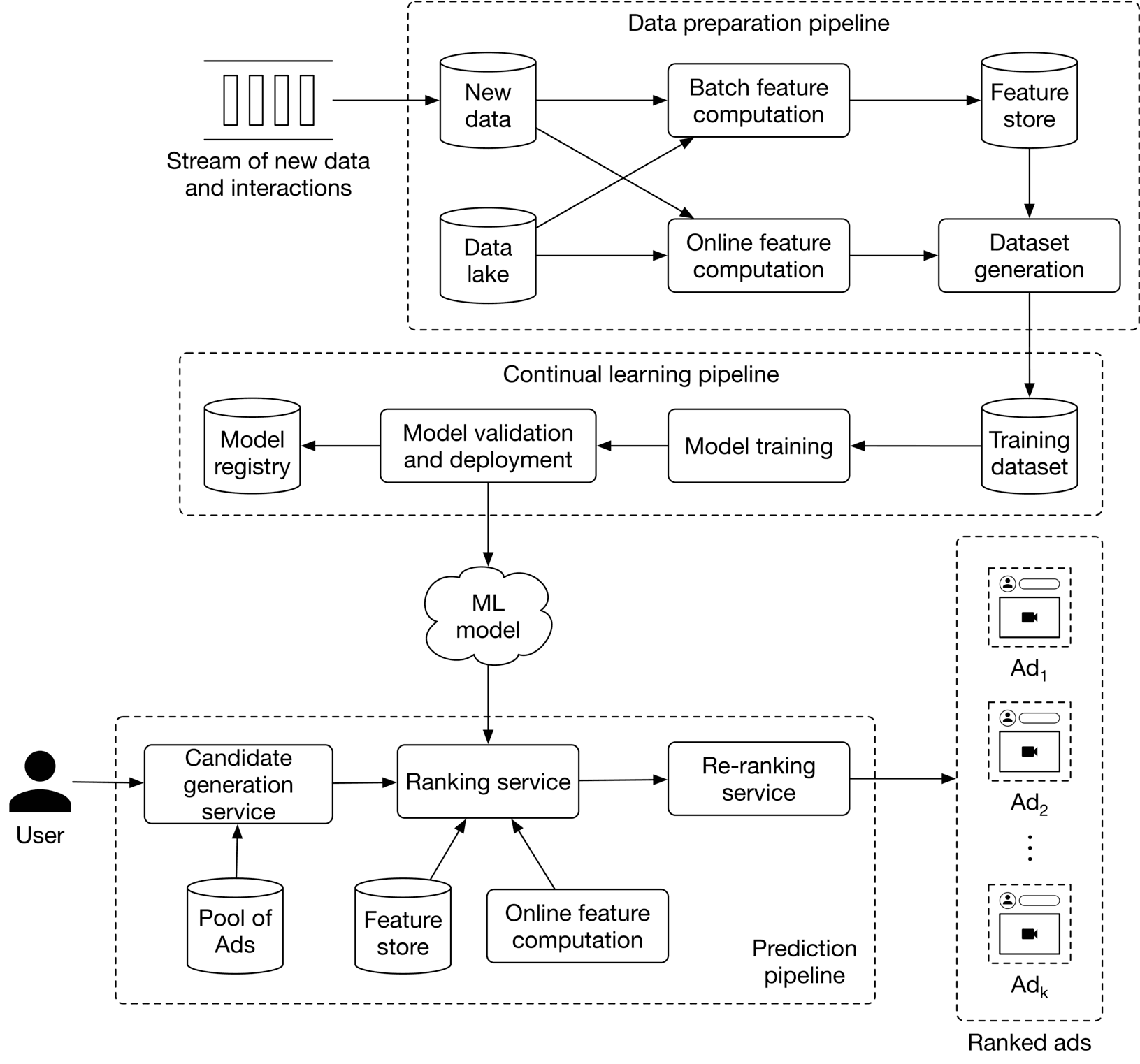 Figure 8.1: Sponsored ads placed on the user’s timeline
In this chapter, we design an (also known as ) system similar to what popular social media platforms use.
Figure 8.1: Sponsored ads placed on the user’s timeline
In this chapter, we design an (also known as ) system similar to what popular social media platforms use.
Clarifying Requirements
Here is a typical interaction between a candidate and an interviewer.
Candidate : Can I assume the business objective of building an ad prediction system is to maximize revenue?
Interviewer: Yes, that’s correct.
Candidate: There are different types of ads, such as video and image ads. In addition, ads can be displayed in different sizes and formats, like users’ timelines, pop-up ads, etc. For simplicity, can I assume ads are placed on users’ timelines only, and every click generates the same revenue?
Interviewer: That sounds good.
Candidate: Can the system show the same ad to the same user more than once?
Interviewer: Yes, we can show an ad more than once. Sometimes, an ad turns into a click after multiple impressions. In reality, companies have a “fatigue period”, that is, they don’t show the same ad to the same user for X days if the user repeatedly ignores it. For simplicity, assume we have no fatigue period.
Candidate: Do we support the “hide this ad” feature? How about “block this advertiser”? These kinds of negative feedback help us to detect irrelevant ads.
Interviewer: Good question. Let’s assume users can hide an ad they don’t like. “Block this advertiser” is an interesting feature, but we don’t need to support it for now.
Candidate: Would it be okay to assume that the training dataset should be constructed using user and ad data, and the labels should be based on user-ad interactions?
Interviewer: Sure.
Candidate: We can construct positive training data points via user clicks, but how do we generate negative data points? Can we assume any impression that is not clicked is a negative data point? What if the user scrolls fast and doesn’t spend time seeing the ad? What if we count an impression as negative, but eventually, the user clicks on it?
Interviewer: These are excellent questions. What are your thoughts?
Candidate: If an ad is visible on a user’s screen for a certain duration but not clicked, we can count it as a negative data point. An alternative approach would be to assume impressions are negative until a click is observed. In addition, we can rely on negative feedback such as “hide this ad” to label negative data points.
Interviewer: Makes sense! In practice, we might use other complex techniques to label negative data points . For this interview, let’s proceed with your suggestions.
Candidate: In ad click prediction systems, it’s critical for the model to learn from new interactions continuously. Is it fair to assume continual learning is a necessity here?
Interviewer: Great point. Experiments have shown that even a 5-minute delay in updating models can damage performance [1].
Let's summarize the problem statement. We are asked to design an ad click prediction system. The business objective of the system is to maximize revenue. The ads are placed only on users' timelines, and each click generates the same revenue. It is necessary to train the model on new interactions continually. We construct the dataset from the user and ad data, and label them based on interactions. In this chapter, we will not discuss AdTech-specific topics as they are not relevant to ML interviews. To learn more about AdTech, refer to [2].
Frame the Problem as an ML Task
Defining the ML objective
The goal of the ad click prediction system is to increase revenue by showing users ads they are more likely to click on. This can be converted into the following ML objective: predicting if an ad will be clicked. This is due to the fact that by correctly predicting click probabilities, the system can display relevant ads to users, which leads to an increase in revenue.
Specifying the system’s input and output
The ad click prediction system takes a user as input, and outputs a ranked list of ads based on click probabilities.
Figure 8.2: Ad click prediction system’s input and output
Choosing the right ML category
Figure 8.2 illustrates how ad prediction can be framed as a ranking problem. As described in Chapter 7, Event Recommendation System, the pointwise Learning to Rank (LTR) is a great starting point for solving ranking problems. The pointwise LTR employs a binary classification model that takes a ⟨\langle⟨ user, ad ⟩\rangle⟩ pair as input and predicts whether the user will click on the ad. Figure 8.3 shows the model's input and output.
Figure 8.3: Binary classification model’s input-output
Data Preparation
Data engineering
Here is some raw data available in this system:
- Ads
- Users
- User-ad interactions
Ads
Ad data is shown in Table 8.1. In practice, we may have hundreds of attributes associated with each ad. For simplicity, we only list important ones.
| Ad ID | Advertiser ID | Ad group ID | Campaign ID | Category | Subcategory | Images or Videos |
|---|---|---|---|---|---|---|
| 1 | 1 | 4 | 7 | travel | hotel | http: //cdn.mysite.com/u1.jpg |
| 2 | 7 | 2 | 9 | insurance | car | http: //cdn.mysite.com/t3.mp4 |
| 3 | 9 | 6 | 28 | travel | airline | http: //cdn.mysite.com/t5.jpg |
| Table 8.1: Ad data |
Users
The schema for user data is shown below.
| ID | Username | Age | Gender | City | Country | Language | Time zone |
|---|---|---|---|---|---|---|---|
| Table 8.2: Schema for user data |
User-ad interactions
This table stores user-ad interactions such as impressions, clicks, and conversions.
| User ID | Ad ID | Interaction type | Dwell time | Location (lat, long) | Timestamp |
|---|---|---|---|---|---|
| 11 | 6 | Impression | 5sec | 38.8951 | |
| -77.0364 | 165845053 | ||||
| 11 | 7 | Impression | 0.4 sec | 41.9241 | |
| -89.0389 | 1658451365 | ||||
| 4 | 20 | Click | - | 22.7531 | |
| 47.9642 | 1658435948 | ||||
| 11 | 6 | Conversion | - | 22.7531 | |
| 47.9642 | 1658451849 | ||||
| Table 8.3: User-ad interaction data |
Feature engineering
Our aim in this section is to engineer features that will assist us in predicting user clicks.
Ad features
Ad features include the following:
- IDs
- Image/video
- Category and subcategory
- Impression and click numbers
Let's examine each in more detail.
IDs
These are advertiser ID, campaign ID, ad group ID, ad ID,etc. Why is it important? The IDs represent the advertiser, the campaign, the ad group, and the ad itself. These IDs are used as predictive features to capture the unique characteristics of different advertisers, campaigns, ad groups, and ads. How to prepare it? The embedding layer converts sparse features, such as IDs, into dense feature vectors. Each ID type has its own embedding layer.
Image/video
Why is it important? A video or image in a post is another signal that can help us predict what the ad is about. For example, an image of an airplane may indicate the ad is related to travel. How to prepare it? The images or videos are first preprocessed. After that, we use a pre-trained model such as SimCLR [3] to convert unstructured data into a feature vector.
Ad category and subcategory
As provided by the advertiser, this is the ad's category and subcategory. For example, here is a list of broad types of categories that are targetable: Arts & Entertainment, Autos & Vehicles, Beauty & Fitness, etc. Why is it important? It helps the model to understand which category the ad belongs to. How to prepare it? These are manually provided by the advertiser based on a predefined list of categories and subcategories. To learn more about preparing textual data, read Chapter 4, YouTube Video Search.
Impressions and click numbers
- Total impression/clicks on the ad
- Total impressions/clicks on ads supplied by an advertiser
- Total impressions of the campaign
Why is it important? These numbers indicate how other users reacted to this ad. For example, users are more likely to click on an ad with a high click-through rate (CTR).
![Image represents a machine learning model architecture diagram illustrating feature concatenation from various sources. The bottom layer shows three feature groups: 'Textual features' \(derived from 'Tokenization' of 'Travel' and 'Flight' categories, processed by a 'Pretrained text model' producing two embedding vectors with numerical values\), 'Engagement features' \(consisting of numerical values representing 'Ad impressions,' 'Ad clicks,' 'Advertiser total clicks,' and 'Campaign total clicks'\), and 'Image/video features' \(processed by a 'Pretrained image/video model' resulting in a visual feature vector\). Each feature group feeds into an 'Embedding' layer, generating a vector of numerical values \(e.g., [-0.8, 0.6, 0, 0.1, -0.3]\). These embeddings, along with the numerical IDs \('Ad ID,' 'Advertiser ID,' 'Campaign ID,' and 'Group ID'\), are then concatenated in the top layer, 'Concatenated features,' forming a combined feature vector for subsequent model processing \(not shown\). The arrows indicate the data flow, showing how individual features are processed and combined to create the final feature vector.](/machine-learning-system-design-interview/images/page07_img17.png) Figure 8.4: Summary of ad-related feature preparation
Figure 8.4: Summary of ad-related feature preparation
User features
Similar to previous chapters, we choose the following features:
- Demographics: age, gender, city, country, etc
- Contextual information: device, time of the day, etc
- Interaction-related features: clicked ads, user's historical engagement statistics, etc
Let's take a closer look at interaction-related features.
Clicked ads
Ads previously clicked by the user. Why is it important? Previous clicks indicate a user's interests. For example, when a user clicks on lots of insurance-related ads, it suggests they are likely to click on a similar ad again. How to prepare it? In the same way as described in "Ad features".
User’s historical engagement statistics
These are the user’s historical engagement numbers, such as their total ad views and ad click rate.
Why is it important? An individual's historical engagement is a good predictor of future engagement. In general, users are more likely to click on ads in the future, if they clicked on ads frequently in the past.
How to prepare it? Engagement statistics are represented as numerical values. To prepare them, we scale their values into a similar range.
Figure 8.5: Feature preparation for user metadata and interactions
Before concluding the data preparation section, let's examine a common challenge in ad click prediction systems. In most cases, these systems deal with lots of high cardinality categorical features. For example, "ad category" takes values from a huge list of all possible categories. Similarly, "advertiser ID" and "user ID" take potentially millions of unique values, depending on how many users or advertisers are active on the platform. Given the huge feature space which often exists, it is common to have thousands or millions of features mostly filled with zeroes. In the model selection section, we will cover techniques to overcome these unique challenges.
Model Development
Model selection
As described in the section "Frame the Problem as an ML Task", the binary classification model is chosen to solve the ranking problem. Binary classifications can be modeled in several different ways. The following are common choices in ad click prediction systems:
- Logistic regression
- Feature crossing + logistic regression
- Gradient boosted decision trees
- Gradient boosted decision trees + logistic regression
- Neural networks
- Deep & Cross networks
- Factorization Machines
- Deep Factorization Machines
Logistic regression (LR)
LR models the probability of a binary outcome using a linear combination of one or multiple features. LR is fast to train and easy to implement. An LR-based ad click prediction system, however, does have the following drawbacks:
- Non-linear problems can't be solved with LR. LR solves the task using a linear combination of input features, which leads to a linear decision boundary. In ad click prediction systems, data is usually not linearly separable, so LR may perform poorly.
- Inability to capture feature interactions. LR is not capable of capturing feature interactions. In ad prediction systems, it is very common to have various interactions between features. When features interact with each other, the output probability cannot be expressed as the sum of the feature effects, since the effect of one feature depends on the value of the other feature.
Given these two drawbacks, LR is not the best choice for the ad prediction system. However, because it is fast to implement and easy to train, many companies use it to create a baseline model.
Feature crossing + LR
To capture feature interactions better, we use a technique called feature crossing
What is feature crossing?
Feature crossing is a technique used in ML to create new features from existing features. It involves combining two or more existing features into one new feature by taking their product, sum, or another combination. It is possible to capture nonlinear interactions between the original features in this way, which can improve the performance of ML models. For example, interactions such as "young and basketball" or "USA and football" may positively impact a model's ability to predict click probability.
How to create feature crosses?
In feature crossing, we manually add new features to the existing features based on prior knowledge. As Figure 8.68.68.6 shows, crossing two features, such as "country" and "language" adds six new features to the existing feature space. To learn more about crossing, refer to [4].
![Image represents a Cartesian product operation between two sets. On the left, we have two feature vectors: `f1: Country` with values `[USA, China, England]` and `f2: Language` with values `[English, Chinese]`. A horizontal line connects these vectors to a central 'x' symbol representing the Cartesian product. This 'x' is labeled 'Country' vertically and 'Language' horizontally, indicating the dimensions of the product. A rightward arrow extends from the 'x' to a list of eight feature vectors \(f3-f8\) on the right. These vectors represent all possible combinations resulting from the Cartesian product of the Country and Language sets: f3 \(USA and English\), f4 \(USA and Chinese\), f5 \(China and English\), f6 \(China and Chinese\), f7 \(England and English\), and f8 \(England and Chinese\). Essentially, the diagram visually demonstrates how combining two sets of features generates a new set containing all possible pairings.](/machine-learning-system-design-interview/images/page07_img18.png) Figure 8.6: Crossing two features: country and language
How to use feature crossing + LR?
As shown in Figure 8.7, feature crossing + LR works as follows:
Figure 8.6: Crossing two features: country and language
How to use feature crossing + LR?
As shown in Figure 8.7, feature crossing + LR works as follows:
- Use feature crossing on the original set of features to extract new features (crossed features)
- Use the original and the crossed features as input for the LR model
Figure 8.7: Feature crossing performed on original features
This method allows the model to capture certain pairwise (second-order) feature interactions. However, it has three shortcomings:
- Manual process: Human involvement is required to choose features to be crossed, which is time-consuming and expensive.
- Requires domain knowledge: Feature crossing requires domain expertise. To determine which interactions between features are predictive signals for the model, we need to understand the problem and the feature space in advance.
- Cannot capture complex interactions: Crossed features may not be sufficient to capture all the complex interactions from thousands of sparse features.
- Sparsity: The original features can be sparse. With feature crossing, the cardinality of the crossed features can become much larger, leading to more sparsity.
Given the drawbacks, this method is not an ideal solution for the ad prediction system.
Gradient-boosted decision trees (GBDT)
We examined GBDT in Chapter 7, Event Recommendation System. Here, we will only explore the pros and cons of GBDT when applied to the ad click prediction system. Pros
- GBDT is interpretable and easy to understand
Cons
- Inefficient for continual learning. In ad click prediction systems, we continuously collect new data such as user, ad, and interaction data. To continually train a model on new data, we generally have two options: 1) training from scratch, or 2) fine-tuning the model on new data. GBDT is not designed to be fine-tuned with new data. So we usually need to train the model from scratch, which is inefficient at a large scale.
- Cannot train embedding layers. In ad prediction systems, it's common to have many sparse categorical features, and the embedding layer is an effective way to represent these features. However, GBDT cannot benefit from embedding layers.
GBDT + LR
There are two steps in this approach:
- Train the GBDT model to learn the task.
- Instead of using the trained model to make predictions, use it to select and extract new predictive features. The newly generated features and the original features are used as input into the LR model for predicting clicks.
Use GBDT for feature selection Feature selection is intended to reduce the number of input features to only those most useful and informative. Using decision trees, we can select a subset of features based on their importance. To better understand how decision trees are used for feature generation, refer to [5].
Use GBDT for feature extraction The purpose of feature extraction is to reduce the number of features by creating new features from existing ones. The newly extracted features are expected to have better predictive power. Figure 8.88.88.8 explains how to extract features using GBDT.
Figure 8.8: Use GBDT for feature extraction
An overview of GBDT in use followed by LR, is shown in Figure 8.9.
Figure 8.9: GBDT + LR overview
Let’s explore the pros and cons of this approach.
Pros:
- In contrast to the existing features, the newly created ones produced by GBDT are more predictive, making it easier for the LR model to learn the task.
Cons:
- Cannot capture complex interactions. Similar to LR, this approach cannot learn pairwise feature interactions.
- Continual learning is slow. Fine-tuning GBDT models on new data takes time, which slows down continual learning overall.
Neural network (NN)
NN is another candidate for building the ad click prediction system. To predict click probabilities using a NN, we have two architectural options:
- Single NN
- Two-tower architecture
Single NN: Using the original features as input, a neural network outputs the click probability (Figure 8.10).
Figure 8.10: NN architecture
Two-tower architecture: In this option, we use two encoders: user encoder and ad encoder. The similarity between ad and user embeddings is used to determine the relevance, that is, the click probability. Figure 8.11 shows an overview of this architecture.
Figure 8.11: Embedding-based NN
Although NNs have many benefits, they may not be the best choice for ad click prediction systems because:
- Sparsity: Given that the feature space is usually huge and sparse, most features are filled with zeroes. It may not be possible for NN\mathrm{NN}NN to learn the task effectively because it does not have access to enough data points.
- Difficult to capture all pairwise feature interactions due to the large number of features.
Given these limitations, we will not use NNs.
Deep & Cross Network (DCN)
In 2017, Google proposed an architecture named DCN [6] to find feature interactions automatically. This addresses the challenges of the manual feature crossing method. The following two parallel networks are used in this method:
- Deep network: Learns complex and generalizable features using a Deep Neural Network (DNN) architecture.
- Cross network: Automatically captures feature interactions and learns good feature crosses.
The outputs of deep network and cross network are concatenated to make a final prediction.
There are two types of DCN architectures: stacked and parallel. Figure 8.128.128.12 shows the architecture of a parallel DCN. To learn more about stacked architecture, refer to [7]. Note that it's not usually expected to provide details of DCN during ML system design interviews. If you are interested in learning more about DCN networks, refer to [7] [8].
Figure 8.12: DCN architecture
DCN architecture is more effective than neural networks because it implicitly learns feature crosses. However, the cross network only models certain feature interactions, which may negatively affect the performance of the cross network model.
Factorization Machines (FM)
FM is an embedding-based model which improves logistic regression by automatically modeling all pairwise feature interactions. In ad click prediction systems, FM is widely used because it can efficiently model complex interactions between features.
So, let's understand how FM works. It automatically models all pairwise feature interactions by learning an embedding vector for each feature. The interaction between two features is determined by the dot product of their embeddings. Let's look at its formula to understand it better:
y^(x)=w0+∑iwixi+∑i∑j⟨vi,vj⟩xixj\hat{y}(x)=w_0+\sum_i w_i x_i+\sum_i \sum_j\langle v_i, v_j\rangle x_i x_jy^(x)=w0+i∑wixi+i∑j∑⟨vi,vj⟩xixj
Where xix_ixi refers to the iii-th feature, wiw_iwi is the learned weight, and viv_ivi represents the embedding of the iii-th feature. ⟨\langle⟨ v_i, v_j ⟩\rangle⟩ denotes the dot product between two embeddings.
This formula may look complex, but it's actually easy to understand. The first two terms compute a linear combination of the features, similar to how logistic regression works. The third term models pairwise feature interactions. Figure 8.138.138.13 shows a high-level overview of FM. Refer to [9] to learn the details of FM.
y^(x)=w0+∑iwixi⏟Logistic regression+∑i∑j⟨vi,vj⟩xixj⏟Pairwise interactions\hat{y}(x)=\underbrace{w_0+\sum_i w_i x_i}{\text{Logistic regression}}+\underbrace{\sum_i \sum_j\langle v_i, v_j\rangle x_i x_j}{\text{Pairwise interactions}}y^(x)=Logistic regressionw0+i∑wixi+Pairwise interactionsi∑j∑⟨vi,vj⟩xixj
Figure 8.13: Factorization Machine architecture
FM and its variants, such as FFM, effectively capture pairwise interactions between features. FM cannot learn sophisticated higher-order interactions from features, unlike neural networks, which can. In the next method, we combine FM and DNN to overcome this.
Deep Factorization Machines (DeepFM)
DeepFM is an ML model that combines the strengths of both NN and FM. A DNN network captures sophisticated higher-order features, and an FM captures low-level pairwise feature interactions. Figure 8.14 shows the high-level architecture of DeepFM. If you are interested to learn more about DeepFM, refer to [10].
Figure 8.14: DeepFM overview
One potential improvement is to combine GBDT and DeepFM. A GBDT converts the original features into more predictive features, while DeepFM operates on the new features. This method has won various ad prediction system competitions [11]. However, adding GBDT to DeepFM negatively affects the training and inference speed, and slows down the continual learning process.
In practice, we usually choose the correct model by running experiments. In our case, we start with a simple LR to create a baseline. Next, we experiment with DCN and DeepFM, as both are widely used in the tech industry.
Model training
Constructing the dataset
For every ad impression, we construct a new data point. The input features are computed from the user and the ad. A label is assigned to the data point, based on the following strategy:
- Positive label: if the user clicks the ad in less than t seconds after the ad is shown, we label the data point as "positive". Note that ttt is a hyperparameter and can be tuned via experimentation.
- Negative label: if the user does not click the ad in less than ttt seconds, we label the data point as "negative".
In practice, companies use more complex methods to find the optimal strategy for labeling negative data points. To learn more, refer to [1].
![Image represents a tabular dataset seemingly used for training a machine learning model, likely for ad click prediction. The table is divided into four columns: a serial number column \(#\), a column for 'User and interaction features' \(represented as a vector of numerical values\), a column for 'Ad features' \(also a numerical vector\), and a 'Label' column indicating whether the data point represents a positive \(ad click\) or negative \(no click\) outcome. Each row represents a single data instance. For instance, row 1 shows a vector of user and interaction features [1, 0, 1, 0.8, 0.1, 1, 0], a vector of ad features [0, 1, 1, 0.4, 0.9, 0], and a positive label. Row 2 similarly presents another data instance with different feature values and a negative label. The numerical values within the feature vectors likely represent different attributes or characteristics of the user, their interaction, and the ad itself. The table structure suggests a supervised learning scenario where the model learns to associate feature vectors with their corresponding positive or negative labels.](/machine-learning-system-design-interview/images/page07_img19.png) Figure 8.15: Constructed dataset
To keep the model adaptive to new data, it must continuously be trained. As a result, new training data points should be continuously generated using new interactions. We will discuss continual learning further in the serving section.
Figure 8.15: Constructed dataset
To keep the model adaptive to new data, it must continuously be trained. As a result, new training data points should be continuously generated using new interactions. We will discuss continual learning further in the serving section.
Choosing the loss function
Since we are training a binary classification model, we choose cross-entropy as a classification loss function.
Evaluation
Offline metrics
Two metrics are typically used to evaluate an ad click prediction system:
- Cross-entropy (CE)
- Normalized cross-entropy (NCE)
CE. This metric measures how close the model's predicted probabilities are to the ground truth labels. CE is zero if we have an ideal system that predicts a 0 for the negative classes and 1 for the positive classes. The lower the CE, the higher the accuracy of the prediction. The formula is:
H(p,q)=−∑c=1CpclogqcH(p, q)=-\sum_{c=1}^C p_c \log q_cH(p,q)=−c=1∑Cpclogqc
where ppp is the ground truth, qqq is the predicted probability, and CCC is the total number of classes.
For binary classification, the CE formula can be rewritten as:
H(p,q)=−∑ipilogqi=−∑i(yilogy^i+(1−yi)log(1−y^i))H(p, q)=-\sum_i p_i \log q_i=-\sum_i\left(y_i \log \hat{y}_i+\left(1-y_i\right) \log \left(1-\hat{y}_i\right)\right)H(p,q)=−i∑pilogqi=−i∑(yilogy^i+(1−yi)log(1−y^i))
where yiy_iyi is the ground truth label of the iii-th data point and y^i\hat{y}_iy^i is the predicted probability of iii-th data point.
Let's take a look at a concrete example, as shown in Figure 8.16.
Figure 8.16: CE of two ML models
Note that aside from using CE as a metric, it is also commonly used as a standard loss function in classification tasks during model training.
Normalized cross-entropy (NCE). NCE is the ratio between our model's CE\mathrm{CE}CE and the CE of the background CTR (average CTR in the training data). In other words, NCE compares the model with a simple baseline which always predicts the background CTR. A low NCE indicates the model outperforms the simple baseline. NCE≥1N C E \geq 1NCE≥1 indicates that the model is not performing better than the simple baseline.
Normalized cross entropy =CE( ML model )CE( Simple baseline )\text { Normalized cross entropy }=\frac{C E(\text { ML model })}{C E(\text { Simple baseline })} Normalized cross entropy =CE( Simple baseline )CE( ML model )
Let's take a look at a concrete example to understand better how NCE is calculated. As shown in Figure 8.17, a simple baseline model always predicts 0.60.60.6 (CTR in the training data). In this case, the NCE value is 0.3240.3240.324 (less than 1), indicating model A outperforms the simple baseline.
Figure 8.17: NCE calculations for model A
Online metrics
Let's examine some metrics we may use during online evaluation.
- CTR
- Conversion rate
- Revenue lift
- Hide rate
CTR. This metric measures the ratio between clicked ads and the total number of shown ads. CTR= Number of clicked ads Number of shown ads C T R=\frac{\text { Number of clicked ads }}{\text { Number of shown ads }}CTR= Number of shown ads Number of clicked ads CTR is a great online metric for ad click prediction systems, as maximizing user clicks on ads is directly related to an increase in revenue. Conversion rate. This metric measures the ratio between the number of conversions and the total number of ads shown. Conversion rate = Number of conversions Number of impressions \text { Conversion rate }=\frac{\text { Number of conversions }}{\text { Number of impressions }} Conversion rate = Number of impressions Number of conversions This metric is important to track as it indicates how many times advertisers actually benefited from the system. This matters because advertisers will eventually lose interest and cease spending on ads if their ads do not lead to conversions. Revenue lift. This measures the percentage of revenue increase over time. Hide rate. This metric measures the ratio between the number of ads hidden by users and the number of shown ads. Hide rate = Number of ads hidden by users Number of shown ads \text { Hide rate }=\frac{\text { Number of ads hidden by users }}{\text { Number of shown ads }} Hide rate = Number of shown ads Number of ads hidden by users This metric is helpful for understanding how many irrelevant ads the system displayed to users, also known as false positives.
Serving
At serving time, the system is responsible for outputting a list of ads ranked by their click probabilities. The proposed ML system design is shown in Figure 8.18. Let's examine each of the following pipelines:
- Data preparation pipeline
- Continual learning pipeline
- Prediction pipeline
Figure 8.18: ML system design
Data preparation pipeline
The data preparation pipeline performs the following two tasks:
- Compute online and batch features
- Continuously generate training data from new ads and interactions
To compute features, the following two options are used: batch feature computation and online feature computation. Let's see how they differ from each other. Batch feature computation Some of the features we chose are static, which means they change very rarely. For example, an ad's image and category are static features. This component computes static features periodically (e.g., every few days or weeks) with batch jobs and then stores the features in a feature store. This improves the system's performance during serving because the features are precomputed. Online feature computation Some features are dynamic as they change frequently. For example, the numbers of ad impressions and clicks are examples of dynamic features. These features need to be computed at query time, and this component is used to compute dynamic features.
Continual learning pipeline
Based on the requirements, continually learning the model is critical. This pipeline is responsible for fine-tuning the model on new training data, evaluating the new model, and deploying the model if it improves the metrics. It ensures the prediction pipeline always uses a model adapted to the most recent data.
Prediction pipeline
The prediction pipeline takes a query user as input and outputs a list of ads ranked by their click probabilities. Since some of the features which the model relies upon are dynamic, we cannot use batch prediction. Instead, requests are served as they arrive using online prediction. As we've seen in previous chapters, a two-stage architecture is used in the prediction pipeline. First, we employ a candidate generation service to efficiently narrow down the available pool of ads to a small subset of ads. In this case, we use the ad targeting criteria often provided by advertisers, such as target age, gender, and country. Next, we employ a ranking model which fetches the candidate ads from the candidate generation service, ranks them based on click probability, and outputs the top ads. This component interacts with the same feature store and online feature computation component. Once the static and dynamic features are obtained, the ranking service uses the model to get a predicted click probability for each candidate ad. These probabilities are used to rank the ads and to output those with the highest click probability. Finally, a re-ranking service modifies the list of ads by incorporating additional logic and heuristics. For example, we can increase the diversity of ads by removing very similar ads from the list.
Other Talking Points
If there is time left at the end of the interview, here are some potential talking points you might discuss with the interviewer:
- In ranking and recommendation systems, it's important to avoid data leakage [12][13][12][13][12][13]
- The model needs to be calibrated in ad click prediction systems. Discuss model calibration and techniques for calibrating a model [14].
- A common variant of FM is a field-aware Factorization Machine (FFM). It's good to talk about FFM and how it differs from FM [15].
- A common variant of DeepFM is XDeepFM. Talk about XDeepFM and how it differs from DeepFM [10].
- We've described why continuous learning is necessary for ad click prediction systems. However, continual learning on new data may lead to catastrophic forgetting. Discuss what catastrophic forgetting is and what common solutions are [16].
References
- Addressing delayed feedback. https://arxiv.org/pdf/1907.06558.pdf.
- AdTech basics. https://advertising.amazon.com/library/guides/what-is-adtech.
- SimCLR paper. https://arxiv.org/pdf/2002.05709.pdf.
- Feature crossing. https://developers.google.com/machine-learning/crash-course/feature-crosses/video-lecture.
- Feature extraction with GBDT. https://towardsdatascience.com/gradient-boosted-decision-trees-explained-9259bd8205af/.
- DCN paper. https://arxiv.org/pdf/1708.05123.pdf.
- DCN V2 paper. https://arxiv.org/pdf/2008.13535.pdf.
- Microsoft’s deep crossing network paper. https://www.kdd.org/kdd2016/papers/files/adf0975-shanA.pdf.
- Factorization Machines. https://www.jefkine.com/recsys/2017/03/27/factorization-machines/.
- Deep Factorization Machines. https://d2l.ai/chapter_recommender-systems/deepfm.html.
- Kaggle’s winning solution in ad click prediction. https://www.youtube.com/watch?v=4Go5crRVyuU.
- Data leakage in ML systems. https://machinelearningmastery.com/data-leakage-machine-learning/.
- Time-based dataset splitting. https://www.linkedin.com/pulse/time-based-splitting-determining-train-test-data-come-manraj-chalokia/?trk=public_profile_article_view.
- Model calibration. https://machinelearningmastery.com/calibrated-classification-model-in-scikit-learn/.
- Field-aware Factorization Machines. https://www.csie.ntu.edu.tw/~cjlin/papers/ffm.pdf.
- Catastrophic forgetting problem in continual learning. https://www.cs.uic.edu/~liub/lifelong-learning/continual-learning.pdf.